
Monte Carlo Simulation
Monte Carlo Simulation
- Last updated
- Jul 22, 2026
- Relationships
- 6
Mental model
Do not bet on one future. Sample many coherent futures, run the full model through each one, and read the distribution.
Visual memory card
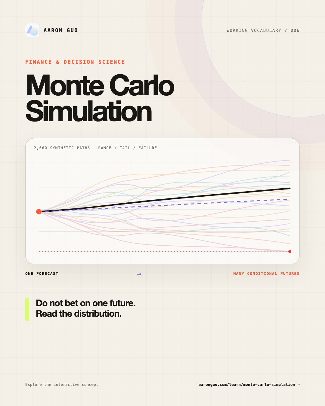
The pattern, in one image.
A compact visual makes the pattern easier to recognize when it appears in a different example.

01 · Conditional futures lab
Change an assumption. Watch the whole distribution move.
Every control is wired into the same 2,000-path model. The dashed line preserves the example assumptions so you can distinguish a real effect from a freshly rescaled chart.
2,000 synthetic paths
The shaded fan contains the middle 80% and 50% of outcomes. Faint lines are sampled paths; the solid line is the current median.
Accurate reading: 71.2% of 2,000 synthetic paths lasted the full horizon under the visible return, volatility, correlation, inflation, fee, timing, and withdrawal assumptions.
Decision setup
Model assumptions · return, volatility, dependence, inflation & fees
These inputs define which synthetic worlds can exist. They are assumptions, not forecasts.
02 · Reading discipline
The chart becomes useful when its limits stay visible.
A range is not a forecast
The fan describes outcomes allowed by the model. It does not identify which path will occur.
More runs solve one error
Iterations reduce sampling noise. They do not repair omitted risks, weak data, or unrealistic distributions.
Compare rules, not destiny scores
Results are strongest for comparing decisions under consistent assumptions and inspecting the paths that fail.
Educational, hypothetical illustration only. It does not provide personalized investment advice or predict actual results.
Monte Carlo Simulation
A single forecast makes uncertainty look like a line. Monte Carlo simulation makes it visible as a distribution.
The method repeatedly samples uncertain inputs, sends each sample through the same model, and records the outcome. One run creates one internally consistent possible world. Thousands of runs reveal a range, a median, tails, thresholds, and the paths that fail.
The crucial word is conditional. The result describes what happened inside the worlds the model was allowed to generate. It is not a claim that the model has discovered the objective probability of your real future.
An outdoor event
Suppose you are planning an outdoor event. A forecast of “22°C on average” is not enough to decide whether to rent a tent.
A more useful exercise is to replay the day thousands of times using plausible temperature, rain, and wind conditions—while keeping their relationships intact. Some versions are warm and clear; others are wet, cold, and windy. You can then ask:
- How often does the event cross the failure threshold?
- How bad is the lower tail?
- Which preparation removes the most fragile outcomes?
Monte Carlo simulation applies this same logic to any model with uncertain inputs. The casino supplied the name; disciplined sampling is the actual idea.
The mechanism
Write the outcome as a model:
Y = f(X₁, X₂, …, Xₖ)
Y is the result you care about. The X values are uncertain inputs. A useful simulation then follows seven steps:
- Name the decision and the success condition. “Assets never run out during 30 years” is testable; “the plan looks good” is not.
- Represent input uncertainty. Define ranges or distributions for returns, demand, prices, growth, costs, inflation, duration, or failure rates.
- Represent dependence. Correlation and causal constraints keep sampled worlds coherent. Individually plausible inputs can form an impossible combination.
- Draw one joint sample. This produces one possible world.
- Run the complete model. Preserve compounding, timing, withdrawals, reinvestment, queues, or whatever makes the path matter.
- Repeat. The outcomes form an empirical distribution.
- Read and challenge the distribution. Report ranges, quantiles, threshold frequency, and failure paths; then change assumptions and add stress tests.
More runs reduce sampling noise inside the chosen model. They do not repair a bad model, missing risk, stale data, or an unrealistic distribution.
A long-horizon funding model
Consider a model that starts with assets B₀, makes an inflation-adjusted withdrawal at the beginning of each year, and then applies that year's net portfolio return:
Bₜ = max(0, [Bₜ₋₁ − W₀(1 + π)ᵗ⁻¹] × [1 + Rₜ − f])
Bₜis the year-end balance.W₀is the first withdrawal.πis inflation.Rₜis the sampled portfolio return.fis the annual fee.
Each run samples a different sequence of stock and bond returns while preserving the assumed relationship between them. The model then follows the full path. If assets cannot meet a withdrawal, that path is classified as depleted.
Suppose 1,640 of 2,000 runs last the full period. The careful statement is:
Under these return, volatility, correlation, inflation, fee, timing, and withdrawal assumptions, 82% of the synthetic paths did not deplete.
It is not “this person has an objective 82% chance of success.” The number is better used to compare rule changes under the same assumptions: lower spending, a different allocation, lower costs, more time, or a flexible withdrawal policy.
This page is educational and does not provide personalized investment advice. The interactive outputs are hypothetical and depend entirely on visible model assumptions.
Why sequence changes the outcome
Without deposits or withdrawals, reordering the same annual returns leaves the final compounded value unchanged. Multiplication does not care about order.
With withdrawals, it does. An early loss reduces the capital base while cash is still leaving the model. A later recovery then compounds on fewer assets. Two paths with the same average return can therefore end very differently.
This is why an average path is often a poor substitute for simulated paths. The average can describe no path that ever occurred, hide temporary depletion, and erase the mechanism that caused failure.
What to read in the output
The mean is rarely enough. A decision-quality readout usually includes:
- Median: the middle simulated outcome, useful as a center but not as a promise.
- Quantile range: for example, the 10th to 90th percentile band.
- Threshold frequency: the share of sampled worlds crossing a defined failure or target line.
- Failure timing: whether problems cluster early, late, or around a particular condition.
- Tail severity: how bad outcomes become after the threshold is crossed.
- Sensitivity: which assumptions most change the result.
A probability without its condition is an invitation to false precision. Good communication keeps the assumptions beside the output.
Where it helps
Monte Carlo simulation is useful when:
- several uncertain inputs jointly drive the result;
- the order and timing of events matter;
- the decision depends on a range, tail, or threshold rather than only an average;
- strategies need to be compared under a common set of assumptions; or
- a closed-form solution is unavailable or hides the path.
Examples extend beyond financial models: project schedules, inventory, reliability, queues, energy demand, insurance losses, and measurement uncertainty.
Where it fails
Garbage in, distribution out
Professional-looking histograms do not make unsupported inputs credible. The hardest work is often defining plausible worlds, not generating random numbers.
False precision
84.7% may only be a more stable estimate of the chosen model's answer. Assumption error can be much larger than Monte Carlo sampling error.
Tail blindness
A thin-tailed distribution that never generates liquidity freezes, jumps, regime changes, or correlation spikes cannot reveal those risks. Add explicit stress tests.
Independence fantasy
Sampling every variable independently can create impossible worlds. Growth, margins, rates, defaults, and asset returns often move together.
Policy omission
Real people and organizations adapt. They may change spending, prices, staffing, financing, inventory, or project scope. A fixed-policy model can understate or overstate resilience.
Objective error
A model can optimize the wrong definition of success. Ending just above zero may still violate liquidity, service, safety, or quality constraints along the path.
Neighboring methods
- Scenario analysis tells a small number of coherent stories. It is easier to explain but covers fewer worlds.
- Stress testing forces named extreme conditions. It complements simulation when modeled tails are incomplete.
- Sensitivity analysis identifies the assumptions worth researching or monitoring. It explains drivers more directly than a distribution alone.
- Historical simulation preserves real combinations from observed periods but cannot show conditions absent from the sample.
- Bootstrap resampling draws from observed data and can preserve some empirical structure, especially with block methods.
- A forecast tries to identify a likely future path. Monte Carlo is usually better at conditional ranges and robustness than at naming the path that will occur.
Remember these five things
- Monte Carlo produces many conditional paths, not one privileged forecast.
- The model, input distributions, dependence, and policy rules define which worlds can exist.
- Read ranges, tails, threshold frequency, and failure paths—not only the average.
- More iterations reduce sampling noise, not model risk.
- Compare decisions under consistent assumptions and pair simulation with sensitivity analysis and stress testing.
Self-test
- Why can a fixed 6% annual return behave differently from random paths averaging 6%?
- What assumptions must accompany a reported “82%” result?
- Which mistake cannot be repaired by increasing the number of simulations?
- When should a named stress test be added even if the simulation has a 5th percentile?
- Which inputs in your model should not be sampled independently?
Further reading
- Metropolis & Ulam (1949), “The Monte Carlo Method”
- National Institute of Standards and Technology · New Tool to Account for Uncertainty
- Financial Industry Regulatory Authority Rule 2214 · Requirements for Investment Analysis Tools
- Certified Financial Planner Board · Core Financial Planning Technologies questionnaire
Relationships
Concept neighbors
Scenario Analysis
narrative methodScenario Analysis
Compares a small set of coherent, interpretable futures instead of systematically sampling a large distribution.
Stress Testing
complementary evidenceStress Testing
Forces a model through named extreme conditions that an assumed distribution may rarely or never generate.
Sensitivity Analysis
diagnostic methodSensitivity Analysis
Shows which assumptions move the answer most; Monte Carlo propagates their joint uncertainty.
Sequence Risk
path-dependent riskSequence-of-Returns Risk
Explains why the order of outcomes matters when withdrawals or other path-dependent cash flows are present.
Bootstrap
sampling mechanismBootstrap Resampling
Resamples observed data and can supply paths to a Monte Carlo model while preserving selected empirical features.
Model Risk
parent riskModel Risk
Covers losses caused by flawed structure, inputs, data, assumptions, or inappropriate use of a model.
Evidence trail